Walking Through A Simple Neural Network - NN3my.1

The singularity is approaching. Everyone understands the power of neural networks. Many understand the conceptual framework behind them. Fewer understanding the technical inner workings and see them as a "black box". How do they learn? What do they learn? Is anything interpretable? Hopefully, I can help demystify neural networks and provide answers to these fundamental questions in a series of posts where I break things down into granular pieces organized in a logical and linear fashion.

For simplicity, I will be using an extremely simple neural network for the first example. Many tutorials jump straight into multi-layered networks (with hidden layers and bias units), but we are doing this from the ground up (and there is PLENTY to learn). So enjoy the ride.

Here, I will also introduce the terminology:

Neural networks take inputs (at the input layer) and transform them into outputs (output layer). In between the input and output layers are several functions and modifications that do the transformative "work". If you can represent your question/task as numbers, it's likely that a neural network can learn meaningful features of your data/trend/pattern/whatever. Neural networks are inspired by the brain itself. The brain takes information (both external and internal), processes it, and transforms it into an action/decision based on how it was "trained" (as well as the preexisting biases molded by millions of years of evolution). Neural networks operate in the same way, but one key difference is that there isn't any preexisting bias or structure molded by evolution. We as researchers must CHOOSE this structure (there is a lot of ongoing research about what types of neural networks are best suited for certain problems). We choose the number of layers, the number of neurons in each layer, the connectivity between layers, the initial weights associated with the neurons, the functions that modify the input values of each neuron, and so on.

Given this simple neural network, let's walk through how information is processed in what's called the forward pass. We can do this even before we know what the "task" of the network is. We simply follow the rules.

Before we get started, whip out a pen and paper! Yes this is a simple example, and even those with a superficial understanding of neural networks can quickly calculate the output as simply the input multiplied by the weight, BUT, I'm purposely being thorough here. This is the general form of how neurons pass information to each other. For those unaware, neurons in a typical deep neural network don't simply accept the input * weight value. That value is first transformed by something called an "activation function". For simplicity, the activation in this example is the identity function (output = input), but some common activation functions include the ReLU and Sigmoid functions which we will go over in later posts.

One more thing before we begin, I use a notation that is personally less confusing to me. When neural networks get dense and it becomes tedious to keep track of every neuron and weight, people typically denote specific neurons with numbers and specific weights with superscripts corresponding to the neuron path (the weight between neuron 3 and 4 would be w34). For my notation, positional information is placed directly above the variable to prevent equating superscripts with exponents. So the neuron corresponding to the final layer has an L above it while the neuron in the previous layer has L-1 above it. You will see this notation throughout this and subsequent posts.

So without further ado, the let's walk through the forward pass:

Now that we have the formula for calculating the network activity, we can apply this to a numerical example. First, we'll initialize the weight with the random value of .7. Using an input value of 1.6, we can calculate the forward pass. The final output is 1.6 * .7 = 1.12.

Imagine that we want our network to learn the trend: output = 1.5 * input. The desired answer would be 1.6 * 1.5 = 2.40. The difference between the desired output and the actual output is the error. Networks learn to update their weights based on an error function (E) (sometimes called loss or cost function), which is a function of the difference* between calculated output (o) and the target output(t). The goal is to update the weights so the error is minimized. We will use the mean squared error (MSE*) as our error function:

The question is, how much should we update the weight based on the error? Intuitively, the weight should change proportionally to how much it affects the error . So we first, need to know how much the error changes with respect to the weight, or: ∂E/∂w (yes calculus!). This is referred to as the gradient. To find the gradient, we must work backwards!

*Throughout this tutorial, I typically represent error as (o - t), but many people typically use (t - o).

*The mean squared error is nice because it always returns a positive value and it penalizes larger errors more strongly. In many cases, you will see 1/2 as a constant in front of the mean squared error. People do this so that when differentiating, it looks "nicer". I don't do that, I'm not a baby, it doesn't matter.

So we've come to the first roadblock for most people when it comes to fully grasping the technical details of a neural network's learning process, back-propagation. Back-propagation, or backprop, is the procedure by which a neural network updates its weights based on the error. The issue is that there are usually a series of functions that lie between the weight and the error. In this case, the error is based on the output of the final layer, which is based on the activation function of the final input, which is based on the output of the previous layer (L-1) as well as the weight. Imagine what the chain would be for a more complicated neural network! Luckily, because of the magical chain-rule, the (derivative) a function with respect to a function with respect to a function...is simply the multiple of the derivative of the composite functions. As we work through the steps, things will become much clearer!

Let's take a moment to internalize what we've calculated. Recall in the forward pass, the final output was 1.12 and the target was 2.40. If we plot the error function, the gradient, and a vertical line corresponding to the output (all functions of the output), we can visualize how these all relate to each other.

Based on where the gradient intercepts the output (-4.096), we know the factor by which we will update the weight! Intuitively, our goal is to descend to the minimum value of the error function. The gradient provides "local" information about the slope of the error function. If the value of the gradient is large, the slope of the error function is steep, meaning there is a good chance that there's still a ways to go before the minimum value is reached. The increment that we move along the error curve is called the learning rate, η. Learning rates are typically small (between .00001 and .1) to avoid overshooting

the path towards the minimum error. Learning happens one straight line at a time!

New weights are updated with the following formula*:

*depending on the error function, this could be written as wold + η * gradient

Here is an example of how different learning rates could effect the gradient decent:

Putting everything together, we can finally do a forward pass, calculate the gradient, and do a backward pass to update the weights based on a learning rate of out choosing, .1.

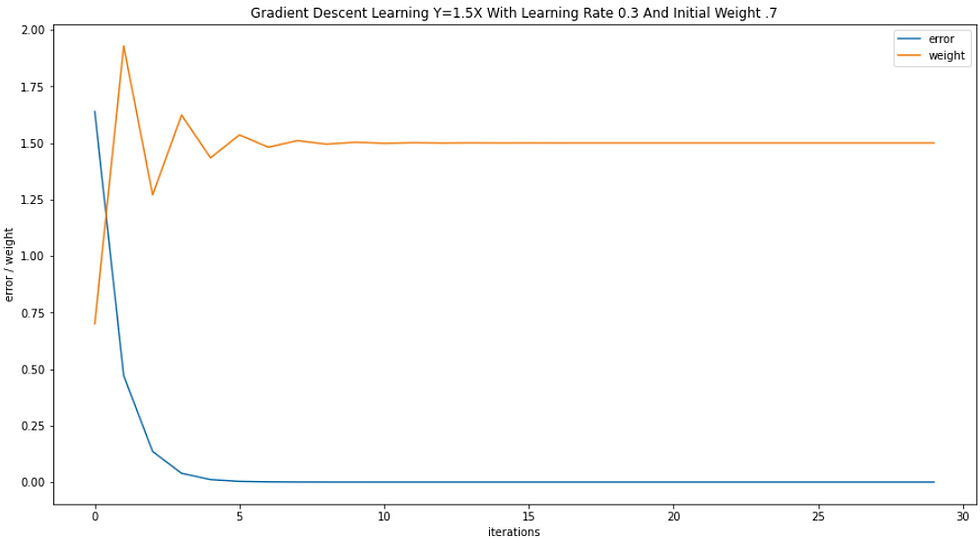
Finally, let's visualize how this simple neural network learns the formula, output = 1.5 x input, with different learning rates (given that it always learns with an input value of 1.6).

learning rate = .1

learning rate = .2

learning rate = .3

learning rate = .4

We see that when the learning rate becomes too high, the gradient shoots far past the bounds of the error function!

So that's as far as we go for this first example. In the next post, we will continue to practice our forward and backward pass calculations on more complicated networks! Hope this was helpful, and remember, neural networks aren't you're enemy (hence the name of this series NNemy ;p).

P.S. If you're in an AI mood and want to read on the history of the field, check out my Science In The News article on the history of AI (or the slightly more in-depth version published in the Weapons of Reason magazine).

-Rockwell